This project is based on undergraduate research I did with the Applied Mathematics Department at Santa Clara University. The code implementation of what is described here can be found on my GitHub.
Specifcally, this work focused on the topic of inverse problems, a rich mathematical field with many relevent applications across all areas of engineering and finding particular pertinence in modern medical imaging systems, computer vision algorithms, remote sensing, and radar to name just a few.
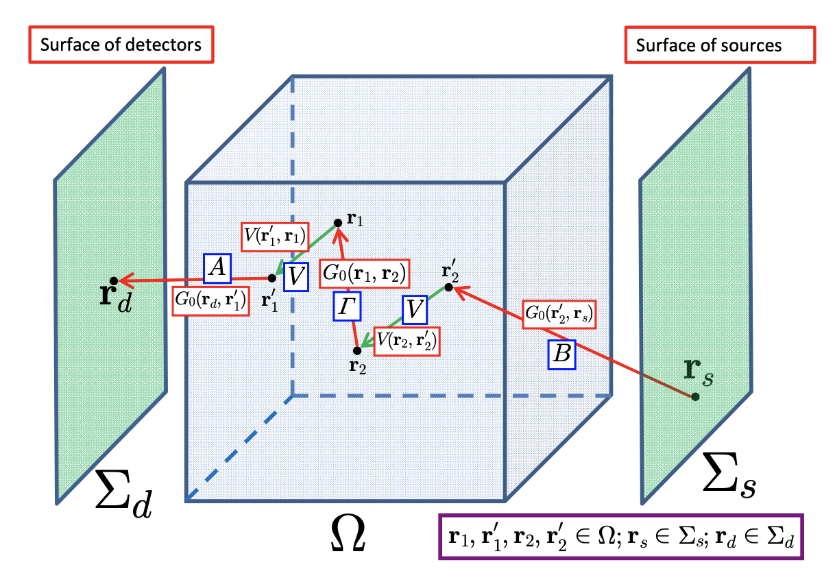 Representation of an inverse problem. Given a known set of sources and set of measurements, determine the material/properties that produced the measured response given the known input 1.
Scattering Theory: The Forward Problem
General Overview
Consider a scalar field \(u(\mathbf{r})\) and the Helmholtz wave equation which describes the propagation of this field in \(\mathbb{R}^{n}\) for \(n\geq2\)
\[[\nabla^{2} + k^{2}\epsilon(\mathbf{r})]u(\mathbf{r}) = -4\pi k^{2}q(\mathbf{r}) \tag{1}\]where \(q(\mathbf{r})\) is the source function and \(\epsilon(\mathbf{r}) = 1\) outside of the bounded domain \(\Omega\) (the sample region). Throughout this paper, the time-harmonic dependence \(e^{j\omega t}\) is suppressed, a single fixed frequency is assumed, and \(k = \omega/c\) is the fixed wave-number, where \(c\) is the velocity of the propagating waves outside of \(\Omega\).
\[[\nabla^{2} + k^{2}]u(\mathbf{r}) = -4\pi k^{2}[\chi(\mathbf{r})u(\mathbf{r}) + q(\mathbf{r})] \tag{2}\]where \(\chi(\mathbf{r}) = \frac{\epsilon(\mathbf{r}) - 1}{4\pi} \tag{3}\) is the susceptibility of the medium.
The total field \(u(\mathbf{r})\) can be decomposed into the sum of incident and scattered fields
\[u(\mathbf{r}) = u_{\textrm{i}}(\mathbf{r}) + u_{\textrm{s}}(\mathbf{r}). \tag{4}\]Note that for this problem, it is assumed that there is no absorption of the incident wave by the scattering medium. This assumption is physically motivated. These methods are often employed to image biological tissue, which is a highly diffusive medium, meaning that an incident field nearly passes through a blocking medium in its entirety, with some slight perturbation due to material properties.
The incident field is assumed to take the form of a plane wave given by
\[u_{\textrm{i}}(\mathbf{r}) = e^{jk\hat{\mathbf{\theta}}\cdot\mathbf{r}} \tag{5}\]where \(\hat{\mathbf{\theta}}\) is a unit vector describing the direction of the incident field. Additionally, the convention used in equation (5) is that a negative term in the exponential indicates outward propagation of the scalar waves. Equation (4) can be transformed to the Lippmann-Schwinger integral equation by inverting the differential operator in the left-hand side of equation 2
\[u(\mathbf{r}) =u_{\textrm{i}}(\mathbf{r}) + k^{2}\int_\Omega G(\mathbf{r, r'}) \chi(\mathbf{r'})u(\mathbf{r'})d^{3}r', \tag{6} \label{eq:Lippmann1}\]where the scattered field is defined as
\[u_{\textrm{s}}(\mathbf{r}) = k^{2}\int_\Omega G(\mathbf{r, r'}) \chi(\mathbf{r'})u(\mathbf{r'})d^{3}r' \tag{7} \label{eq:scattered-field}\]The Born Series
Motivation
Equation (6) has an unknown under the integral in the right-hand side, which is known as an integral equation. In order to solve for the total field, some assumptions must be made. First, it is assumed that the system exhibits weak scattering when illuminated with an incident field. This means that \(u_{\textrm{s}}(\mathbf{r}) << u_{\textrm{i}}(\mathbf{r}) \tag{8} \label{eq:weak-scattering}\)
which indicates that the incident field and the scattered field are not that different. In other words, the sample does not add much distortion to the total field of the system. This allows the integral equation in (6) to be iterated on using a simple fixed-point iteration method. This leads to the Born Series expansion for the total field of this system.
The Born Series Expansion
Under the assumption weak scattering, equation (6) can be solved for in terms of the incident field alone. This results in \(u(\mathbf{r}) =u_{\textrm{i}}(\mathbf{r}) + k^{2}\int_\Omega G(\mathbf{r, r'}) \chi(\mathbf{r'})u_\mathrm{i}({\mathbf{r'}})d^{3}r'. \tag{9} \label{eq:Lippmann2}\) Applying a fixed-point iteration to this equation results in the well-known Born Series
\[u(\mathbf{r}) =u_{\textrm{i}}(\mathbf{r}) + k^{2}\int_\Omega G(\mathbf{r, r'}) \chi(\mathbf{r'})u_\mathrm{i}({\mathbf{r'}})d^{3}r'\] \[+ k^{4}\int_{\Omega\times\Omega} G(\mathbf{r, r'}) \chi(\mathbf{r'}) G(\mathbf{r',r''}) \chi(\mathbf{r''})u_\mathrm{i}({\mathbf{r''}}) d^{3}r' d^{3}r'' +\ldots \tag{10} \label{eq:Born-Series}\]Equation (10) will be referred to as the Born series, and the approximation to u that results from keeping only the linear expansion in \(\chi\) is the Born approximation.
Now, for the sake of neatness we define an integral operator in order to apply to the Lippmann-Schwinger equation. The integral operator \(G\) which applies the following to a function \(f\)
\[Gf = \int G(\mathbf{r, r'}) f(\mathbf{r'})dr'. \tag{11} \label{eq:G_operator}\]This will make the resulting Born series expansion take on a familiar and easy form to work with when the numerical implementation is discussed. Additionally, we let the quantity \(V = k^2\chi\). Using the operator notation given in equation (11), (6) can be expressed as
\[u = u_\mathrm{i} + GVu_\mathrm{i} + (GV)^2u_\mathrm{i} + (GV)^3u_\mathrm{i} + \ldots \\\] \[= (I + GV + (GV)^2 + (GV)^3 +\ldots)u_\mathrm{i}. \tag{12} \label{eq:operator_Born-Series}\]To analyze the convergence of the Born series, let the application of each successive scattering term operator (\((GV)^n\)) be denoted as
\[\kappa = I + GV + (GV)^2 + (GV)^3 +\ldots,\]which will converge if \(\|\kappa\|< 1\) in any suitable norm. For an arbitrary selection of norm,
\[\|\kappa\| = \|I + GV + (GV)^2 + (GV)^3 +\ldots\| \\ \leq \|I\| + \|GV\| + \|(GV)^2\| + \|(GV)^3\| +\ldots \\\] \[= \sum_{i=0}^{\infty}\|GV\|^i = (I-GV)^{-1}. \tag{13} \label{eq:convergence_Born-series}\]Note that convergence only occurs provided that \(\|GV\|<1\) (in any norm) because equation (13) is a geometric series with common ratio \(GV\). Using this result, we can express the total field \(u(\mathbf{r})\) as
\[u(\mathbf{r}) = (I-GV)^{-1}u_\mathrm{i}. \tag{14} \label{eq:utot-by-born}\]A physical interpretation of this result is the following: given an observation point located at \(\mathbf{r} \in \mathbb{R}^3\), equation (14) gives the sum of all orders of scattering from each point in the scattering medium, to the detector. An incident field into the scattering medium could “scatter once” off a single point in the medium, or it can “internally scatter” in the medium before exiting. The result in equation (14) gives the sum of all orders, meaning it accounts for single scattering, double scattering, and so on.
Modeling the Forward Problem
The goal of this section is to explain how the forward problem given by the Born series expansion in (13) is numerically modeled.
Discretization
For a given sample region, with some scattering object of interest inside of it, a suitable discretization scheme needs to be developed in order to solve for the scattered field at a detector location. To start, the sample space of interest is defined to be the unit cube, with dimensions
\[0\leq x \leq 1\] \[0\leq y \leq 1\] \[0\leq z \leq 1.\]The sample space has a material index of \(0\), and it is assumed to be free-space. Within the sample region is the scatterer, which is a cube of dimensions
\[0.25\leq x \leq 0.75\] \[0.25\leq y \leq 0.75\] \[0.25\leq z \leq 0.75\]Within the scattering region, the material index \(\chi\) is defined and is non-zero. The sample-region (with the scattering medium included) is discretized into cubic voxels \(\mathbb{C}_{\ell}\left(n=1, \ldots, N_{v}\right)\) of volume \(h^3\) each, where \(h\) is the discretization step and \(N_{v}\) is the total number of voxels.
We then make the following approximation:
\(\chi(\mathbf{r})=\chi_{\ell} \quad \text { AND } \quad u(\mathbf{r})=u_{\ell} \quad \text { IF } \quad \mathbf{r} \in \mathbb{C}_{\ell}. \tag{15}\) This approximation cannot hold for all values of \(\mathbf{r}\), however, by restricting attention to the centers of the respective voxels \(\mathbb{C}_{\ell}\), we get an expression for the scattered field:
\[u_{\textrm{s}}(\mathbf{r}) = \int_\Omega G(\mathbf{r, r'}) V(\mathbf{r'})u(\mathbf{r'})d^{3}r' = \sum_{\ell=1}^{n}\int_{\mathbb{C}_{\ell}}G(\mathbf{r, r'}) V(\mathbf{r'})u_{\mathrm{i}}(\mathbf{r'}) d^{3}r'\] \[= \sum_{\ell=1}^{n}V(\mathbf{r'}_{\ell}^{\textrm{m}})u_{\mathrm{i}}(\mathbf{r'}_{\ell}^{m})\int_{\mathbb{C}_{\ell}} G(\mathbf{r, r'}) d^{3}r', \tag{16} \label{eq:uscatt-dicr}\]where \(\mathbf{r'}_{\ell}^{\textrm{m}}\) denotes the midpoint of the \(\ell^{\mathrm{th}}\) voxel.
Evaluating the Green’s function under the in (16) is done by a midpoint quadrature rule under two circumstances: evaluation at different voxel, and evaluation at the same voxel. The latter case is known as singularity treatment. For the case where the cells are different (\(\ell \neq p\)) the integral is taken to be
\[\int_{\mathbf{r} \in \mathbb{C}_{\ell}} G_{0}\left(\mathbf{r}_{\ell}^{\textrm{mid}}, \mathbf{r}\right) d^{3} r \approx h^{3} G_{0}\left(\mathbf{r}_{\ell}^{\textrm{mid}}, \mathbf{r}_{p}^{\textrm{mid}}\right), \quad \ell \neq p. \tag{17}\]For \(\ell=p\), a singularity occurs and a treatment method must be applied. For this scenario, the Green’s function is evaluated as
\[\int_{\mathbf{r} \in \mathbb{C}_{\ell}} G_{0}\left(\mathbf{r}_{\ell}^{\textrm{mid}}, \mathbf{r}\right) d^{3} r \approx (k h)^{2}(\xi+i k h) \tag{18}\]where
\[\xi=\log (26+15 \sqrt{3})-\pi / 2 \approx 2.38. \tag{19}\]Applying this discretization and quadrature scheme to the forward problem at hand, we can express the scattered field in terms of a product of vectors and matrices.
Walk-through of the Code
The current code that was completed this summer models the forward scattering problem based upon the theory and approximations explained above. The code is compartmentalized into different programs and sub-functions for speed and testing purposes.
The file forwardScat_3D.m is the “main” program file which does the discretization and matrix evaluation for the forward scattering problem. This program calls the sub-functions createSources.m, createDetectors.m, _detectorFields.m, and greensMatrix.m. Within the main file forwardScat_3D.m, the number of incident plane waves is first specified. Additionally, the incident direction of the waves is controllable by selection of the \(\phi\) and \(\theta\) combinations, which are the azimuthal and elevation angles of a spherical coordinate system, respectively. Next, the scattering potential is declared, with an arbitrary constant, homogeneous value of the susceptibility defined using the rho variable. After this, the detectors are initialized along a uniform grid with a specified number of detectors in the x and y directions, held at a fixed value of z outside of the scattering region. Finally, the interaction matrix is computed to define the scattering behavior between every point in the scattering region. After all these steps are completed, the scattered field is computed using matrix multiplication, and the results are saved into a struct for further post-processing.
The struct stored after running forwardScat_3D.m is used in the file firstBorn_recovery.m in order to model the linear inverse problem. As a reminder, the linear inverse problem is simply the inversion of the first order Born-series expansion in equation (10). In order to cross-check the results and assure a suitable recovery is made using the linear inversion, the recovered material matrix found by the first-Born inversion is plotted using the imagesc() function in MATLAB. The result is shown here:
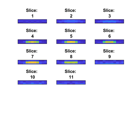 Material recovery by inversion of the first-Born approximation for the scattered field.
We see that the resulting cross-sections are somewhat “noisy” and spread out. This has to do with the condition number of the matrix constructed in the firstBorn_recovery.m, along with the fact that only the first order of the born series is considered.
Sources
Levinson HW, Markel VA. Solution of the nonlinear inverse scattering problem by T-matrix completion. II. Simulations. Phys Rev E. 2016 Oct;94(4-1):043318. doi: 10.1103/PhysRevE.94.043318. Epub 2016 Oct 25. PMID: 27841565. ↩