Method of Moments Antenna Simulator

Introduction: What is Method of Moments?

The Method of Moments is a technique used to solve Maxwell’s Equations in the frequency domain. In the MoM, electromagnetic sources are the quantities of interest, and as such MoM is extremely useful for solving radiation and scattering problems. The Method of Moments converts an integral equation relating the known electric field incident onto a conducting object in terms of unknown source currents induced on the conducting object into a linear system which can be solved numerically. MoM excels at solving problems involving systems made of metal or PEC (Perfect Electric Conductor, \(\sigma = \infty\) ) in free space. This project investigates the scattered fields produced by a \(\lambda/2\) dipole antenna operated at 2.5 GHz. In particular, the validity of Method of Moments for this structure is displayed through calculation of known properties of \(\lambda/2\) dipole antennas such as the input impedance at the antenna feed and the current distribution on the antenna. This post will cover the theoretical background of the Method of Moments, and highlight an example implementation.The full code for this implementation can be found on my GitHub.

Foundations

An incident electric field on a PEC object or other conducting body induces currents on that object which in turn result in scattered electric fields. The system can be represented by the following diagram

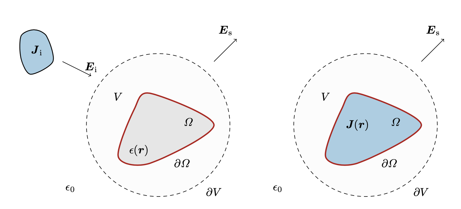Electric field scattering off a conducting body ¹.

Figure 1 displays the scattered field given some incident electric field. Given a current distribution \(\mathbf{J(r')}\) induced on the conducting body, the scattered field can be solved for in terms of the current via the Dyadic Green’s Function. This is know as the Electric Field Integral Equation (EFIE) and is given by

\[\mathbf{E_{sc}(r)} = \int_\Omega \mathbf{G(r, r')}\cdot\mathbf{J(r')}\mathbf{dr'} \tag{1}\]

where \(\mathbf{G(r, r')}\) is the Dyadic Greens Function and \(\mathbf{J(r')}\) is the current induced on the object’s surface \(\Omega\). If the object is known to be PEC, then Maxwell’s Equations can be simplified by boundary conditions. On the surface of a PEC object, the electric field must be normal to the surface, which also means there must be no tangential component. Given this, the total electric field on the surface of the object can be given by

\[\mathbf{E(r)} = \mathbf{E_{sc}(r)} + \mathbf{E_{i}(r)} \tag{2}\]

Considering only the tangential component on the surface of the object, (2) can be reduced to

\[\mathbf{\hat{n}\times E(r)} = \mathbf{\hat{n}}\times\mathbf{E_{sc}(r)} + \mathbf{\hat{n}}\times\mathbf{E_{i}(r)} = 0 \tag{3}\] \[\mathbf{\hat{n}}\times\mathbf{E_{i}(r)} = -\mathbf{\hat{n}}\times\mathbf{E_{sc}(r)} \quad \forall \mathbf{r}\in\Omega \tag{4}\]

Making a substitution of the above we arrive at the following integral equation

\[\mathbf{\hat{n}}\times\mathbf{E_{i}(r)} = -\mathbf{\hat{n}}\times\int_\Omega \mathbf{G(r, r')}\cdot\mathbf{J(r')} \mathbf{dr'} \quad \forall \mathbf{r}\in\Omega \tag{5}\]

The goal of Method of Moments is to massage this integral equation into a matrix form so it can be solved numerically. This can be done by noticing that in (3), \(\mathbf{E_{i}(r)}\) is known, \(\mathbf{G(r, r')}\) is an operator, and \(\mathbf{J(r')}\) is unknown. This form can be expressed as an operator equation by

\[g = \mathscr{L}f \tag{6}\]

where \(g\) is a known output function, \(\mathscr{L}\) is a linear operator, and \(f\) is an unknown function. This means (4) takes the form

\[\mathbf{\hat{n}}\times\mathbf{E_{i}(r)} = -\mathbf{\hat{n}}\times\mathscr{L}\mathbf{J(r')} \quad \forall \mathbf{r}\in\Omega \tag{6}\]

Drawing the parallel between (5) and (6) is the key to setting up a system using the Method of Moments. Once this is established, the unknown function can be expanded using a reasonably complete basis provided we know what the basis functions should look like. That will be explained shortly. For now, we must turn $\mathbf{E_{sc}(r)}$ into something we can work with.

Without going through the derivation, it can be shown that the Dyadic form of $\mathbf{E_{sc}(r)}$ is given by

\[\mathbf{E_{sc}(r)} = -j\omega\mu\int_{\Omega'} G_0(\boldsymbol{r},\boldsymbol{r}')\mathbf{J(r')} + \frac{1}{k^2}\nabla G_0(\boldsymbol{r},\boldsymbol{r}')\nabla'\cdot\mathbf{J(r')}\mathbf{dr'} \tag{7}\]

where \(\omega,\mu,k, G_0(\boldsymbol{r},\boldsymbol{r}')\) are the radial frequency, magnetic permeability of free-space, wave-number, and scalar free space Green’s function, respectively. Additionally, the primed coordinates represent the source locations, and operators with primes on them only act on source functions.

Now that we have the form for the scattered fields, the unknown current distribution $\mathbf{J(r’)}$ must be expanded into a series of known basis functions. This takes the form

\[\mathbf{J(r')} = \sum_{n=1}^{N} I_n\mathbf{\boldsymbol{\psi_n}(r')} \tag{8}\]

where \(\mathbf{\boldsymbol{\psi_n}(r')}\) is a known basis function, and \(I_n\) are the unknown current expansion coefficients. A reasonably complete, simple, and natural choice of basis functions are piece-wise, linear roof-top basis functions shown as:

![basis_function]basis_funcs.png){: width=”500” height=”4000” } Roof-top basis function on a meshed-wire structure.

The details of this basis function will be explained later during the description of implementation. For now it is important to note that they are piece-wise linear, the value at the center node is $1$, and the middle value of either side of the basis function is $0.5$.

These basis functions are selected such that they pick off the tangential component of the electric field, so moving forward the \(\hat{n}\times\) can be dropped. Substituting (8) into (3) and dropping the \(\hat{n}\times\) we get

\[\mathbf{E_{i}(r)} = Z_0\sum_{n=1}^{N} I_njk\int_{\Omega'} G_0(\boldsymbol{r},\boldsymbol{r}')\boldsymbol{\psi_n}(r') + \frac{1}{k^2}\nabla G_0(\boldsymbol{r},\boldsymbol{r}')\nabla'\cdot\boldsymbol{\psi_n}(r')\mathbf{dr'} \tag{9}\]

In the wire-antenna system, a wire is decomposed into a mesh, and a basis function is defined on each segment pair. Since each little truncated piece of the wire antenna acts like an even smaller antenna, we would like a metric to determine how each basis function interacts with one another. This can be done via inner-product testing, and the testing method used for MoM is done using Galerkin’s Method. Galerkin’s method takes the strong-form representation of the field given in (9) and converts it into a weak form. The testing function used for this process will be the same basis function used to describe currents on the wire. Testing each side of (9) with a basis function describing a different section of current \(\mathbf{\boldsymbol{\psi_m}(r)}\) and rearranging the expression using integration by parts we get

\[\langle \mathbf{\boldsymbol{\psi_m}(r)}, \mathbf{E_{i}(r)}\rangle = \int_{\Omega}\mathbf{\boldsymbol{\psi_m}(r)}\cdot\mathbf{E_{i}(r)}\mathbf{dr'}\] \[= Z_0\sum_{n=1}^{N} I_njk\int_{\Omega} \int_{\Omega'} \mathbf{\boldsymbol{\psi_m}(r)}\cdot\boldsymbol{\psi_n}(r')G_0(\boldsymbol{r},\boldsymbol{r}') - \frac{1}{k^2}\nabla\cdot\mathbf{\boldsymbol{\psi_m}(r)}\nabla'\cdot\boldsymbol{\psi_n}(r')G_0(\boldsymbol{r},\boldsymbol{r}')\mathbf{dr'}\mathbf{dr} \tag{10}\]

Finally, we can put this form given by (10) into our operator equation form. We let

\[V_m = \int_{\Omega}\mathbf{\boldsymbol{\psi_m}(r)}\cdot\mathbf{E_{i}(r)}\mathbf{dr} \tag{11}\]

and we let

\[Z_{mn} = jkZ_0\int_{\Omega} \int_{\Omega'} \mathbf{\boldsymbol{\psi_m}(r)}\cdot\boldsymbol{\psi_n}(r')G_0(\boldsymbol{r},\boldsymbol{r}') - \frac{1}{k^2}\nabla\cdot\mathbf{\boldsymbol{\psi_m}(r)}\nabla'\cdot\boldsymbol{\psi_n}(r')G_0(\boldsymbol{r},\boldsymbol{r}')\mathbf{dr'}\mathbf{dr} \tag{12}\]

We can express the system as

\[V_m = \sum_{n=1}^{N} Z_{mn}I_n \tag{13}\]

Collecting \(N\) of of these expressions for each basis function allows for the well-known matrix representation given by

\[\mathbf{V} = \mathbf{ZI} \tag{14}\]

where \(\mathbf{V}\) is incident electric field projected onto the basis (can be seen as an incident voltage), \(\mathbf{Z}\) is the Impedance Matrix representation of the Dyadic Green’s Function integral operator acting onto the basis, and \mathbf{I} are the unknown currents projected onto the basis.

Equation (14) is the form we desired to massage equation (4) into, and since it is in matrix form it allows us to easily solve for the unknown currents and study interesting properties of the system.

MoM: Numerical Implementation

Solving the system \(\mathbf{V} = \mathbf{ZI}\) really comes down to solving for the Impedance Matrix. This is done by splitting the expression into the the corresponding scalar field and potential field matrices. This is done as follows. Let a vector potential \(\mathbf{A}\) be defined as

\[\mathbf{A} = \int_{\Omega} \int_{\Omega'} \mathbf{\boldsymbol{\psi_m}(r)}\cdot\boldsymbol{\psi_n}(r')G_0(\boldsymbol{r},\boldsymbol{r}')\mathbf{dr'}\mathbf{dr} \tag{15}\]

and let a scalar potential field \(\boldsymbol{\Phi}\) be defined as

\[\boldsymbol{\Phi} = \int_{\Omega} \int_{\Omega'} \nabla\cdot\mathbf{\boldsymbol{\psi_m}(r)}\nabla'\cdot\boldsymbol{\psi_n}(r')G_0(\boldsymbol{r},\boldsymbol{r}')\mathbf{dr'}\mathbf{dr} \tag{16}\]

This decomposition allows the Impedance Matrix to be represented as

\[\mathbf{Z_{mn}} = jkZ_0(\mathbf{A_{mn}} - \frac{1}{k^2}\boldsymbol{\Phi_{mn}}) \tag{17}\]

Calculating the Impedance Matrix of the system comes down to finding these vector and scalar potential fields. Let’s first solve for the potential field \(\boldsymbol{\Phi_{mn}}\) by analyzing the divergence terms \(\nabla\cdot\mathbf{\boldsymbol{\psi_m}(r)}\) and \(\nabla'\cdot\boldsymbol{\psi_n}(r')\). The divergence is the rate of change of a vector along the direction it points, which for our basis functions corresponds to the slope of a linear function with respect to the wire length. We can see from Figure 2 that each basis function is piece-wise linear with positive a positive slope on the \(\ell_{n}^-\) segment and a negative slope on the \(\ell_{n}^+\) segment. This means the divergence of a basis function is given as

\[\nabla\cdot\mathbf{\boldsymbol{\psi_i}} = \frac{\partial \Phi_{i}^+}{\partial \ell} = -\frac{1}{S_{i}^+} \quad \forall\mathbf{r}\in\ell_{m}^+ \tag{18}\] \[\nabla\cdot\mathbf{\boldsymbol{\psi_i}} = \frac{\partial \Phi_{i}^-}{\partial \ell} = \frac{1}{S_{i}^-} \quad \forall\mathbf{r}\in\ell_{m}^- \tag{19}\]

where \(S_i\) is the length of the segment over which the basis function is defined. These divergence values are constant and can be pulled out of the \(\boldsymbol{\Phi_{mn}}\) integral. Note that since basis functions are piece-wise linear, and there are two basis functions per impedance matrix calculation, that means there are $4$ total integrals that must be calculated. For the scalar potential matrix that corresponds to \(\boldsymbol{\Phi_{mn}} = \boldsymbol{\Phi_{mn}^{++}} + \boldsymbol{\Phi_{mn}^{+-}} + \boldsymbol{\Phi_{mn}^{-+}} + \boldsymbol{\Phi_{mn}^{--}}\) . If we consider the \(\boldsymbol{\Phi_{mn}^{++}}\) then this integral becomes

\[\boldsymbol{\Phi_{mn}^{++}} = \frac{-1}{S_{m}^+}\frac{-1}{S_{n}^+}\int_{\ell_{m}^+}\int_{\ell_{n}^+}G_0(\boldsymbol{r},\boldsymbol{r}')\mathbf{dr'}\mathbf{dr} \tag{20}\]

We can evaluate this integral by quadrature. Since our function is simple and the interval is small, simple midpoint quadrature rule will be sufficient to solve this. The midpoint quadrature rule is given by

\[\int_\ell f(x)dx \approx |\ell|f(x_m) \tag{21}\]

where \(x_m\) is the midpoint of the integration domain \(\ell\). Applying this rule to (20) reduces the equation to

\[\boldsymbol{\Phi_{mn}^{++}} = \frac{-1}{S_{m}^+}\frac{-1}{S_{n}^+}{S_{n}^+}{S_{m}^+}G_0(\boldsymbol{r}_m^+,\boldsymbol{r}_m^+) = G_0(\boldsymbol{r}_m^+,\boldsymbol{r}_m^+) \tag{21}\]

The same process can be applied to the othe three cases, but the signs will be different. A near identical process applies to solving \(\mathbf{A}\), however there is a dot product term as well as some additional scaling due to evaluation of the basis functions at their midpoints. Considering the \(\mathbf{A_{mn}^{++}}\) term, we get that

\[\mathbf{A_{mn}^{++}} = \int_{\ell_{m}^+}\int_{\ell_{n}^+}\mathbf{\boldsymbol{\psi_m}(r)}\cdot\boldsymbol{\psi_n}(r')G_0(\boldsymbol{r},\boldsymbol{r}')\mathbf{dr'}\mathbf{dr}\] \[= \mathbf{\hat{a}_m^+}\cdot\mathbf{\hat{a}_n^+}\int_{\ell_{m}^+}\int_{\ell_{n}^+}\psi_m^+(\mathbf{r})\psi_n^+(\mathbf{r'})G_0(\boldsymbol{r},\boldsymbol{r}')\mathbf{dr'}\mathbf{dr}\] \[\mathbf{A_{mn}^{++}} = \frac{\mathbf{\hat{a}_m^+}\cdot\mathbf{\hat{a}_n^+}{S_{m}^+}{S_{m}^+}}{4}G_0(\boldsymbol{r}_m^+,\boldsymbol{r}_m^+) \tag{22}\]

Again, the same expressions can be derived for the other components of the vector potential integral.

Singularity Treatment

The Free-Space Scalar Green’s Function $G_0(\boldsymbol{r},\boldsymbol{r}’)$ is given by

\[G_0 = \frac{e^{-jk|\mathbf{r-r'}|}}{4\pi|\mathbf{r-r'}|} \tag{23}\]

When \(\mathbf{r}\) is very close or equal to \(\mathbf{r'}\), then a singularity occurs since the Green’s Function will result in division by zero. To get around this in the MoM code, a Thin-Wire Approximation is made. Using this thing-wire approximation, whenever a singularity occurs during computation of a Green’s Function, the $$\G$o$ term is replaced by

\[G_o(\mathbf{r},\mathbf{r'})\rightarrow \frac{1}{s^2}\int_\ell\int_\ell\frac{e^{-jk|\mathbf{r-r'}|}}{4\pi|\mathbf{r-r'}|}\mathbf{dr'}\mathbf{dr} = \frac{1}{2\pi s}\left[\ln{\frac{s}{a}+\sqrt{1+\frac{s^2}{a^2}}}-\sqrt{1+\frac{a^2}{s^2}}+\frac{a}{s}\right] - \frac{jk}{4\pi} \tag{24}\]

where \(a\) is the wire radius and \(s\) is the length of the segment causing the singularity. To implement this in the code, each Green’s Function must be evaluated for singularities and then replaced by (25).

MATLAB Setup

The MATLAB code implemented is suitable for straight-wire dipole antennas of any length. The process begins by making a parameterized curve for the wire of interest. For a straight wire dipole, this curve is characterized by the number of nodes, location of each node, number of segments, and the length of each segment. From this meshing, the basis functions can be defined over each node (excluding the endpoints) and pair of corresponding right/left nodes. Each basis function can be characterized in terms of the number of basis functions, the indices of the $+$ and $-$ segments, the unit vectors \(\mathbf{\hat{a}_m^+}p\) and \(\mathbf{\hat{a}^-}\), and location of the of the unit vectors. Once the meshing and basis function structures are defined, the Impedance Matrix can be calculated, and the resulting characteristics of the antenna being studied can be evaluated.

As an example, I have setup my code to work for a \(\lambda/2\) wire-dipole antenna with a resonance frequency of 2.5 GHz. It is well-known that for a \(\lambda/2\) dipole antenna, at resonance (where the the reactive component of the antenna input impedance is zero \(\rightarrow Imag(Z{in}) = 0\), the radiation resistance of the antenna $R_r$ is around 73 \(\Omega\). In practice, the true resonance at the frequency of interest occurs at around \(0.475\lambda\), so the code is structured such that the parameterized curve has a length a little less than \(\lambda/2\) . For a \(\lambda/2\) dipole, the current distribution is a half-cycle of a sine-wave. The verification of the radiation resistance \(R_r\) at resonance and the current distribution is verified as a benchmark for the MoM code.

Current Distribution Calculation

To model the voltage at the center feed point of the wire, a delta-gap source is used. The following image depicts the setup.

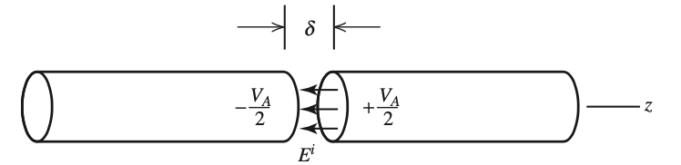Delta-Gap source at the center of the straight-wire dipole ².

This setup corresponds to an incident voltage vector \(\mathbf{V}\) with entries of all zeros except at the center of the wire, which is the middle basis function. Defining this matrix allows for the calculation of \(\mathbf{I}\). We expect the current distribution to be a half-sine wave as stated earlier, and it should look as follows:

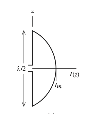Current distribution on a half-wave dipole ².

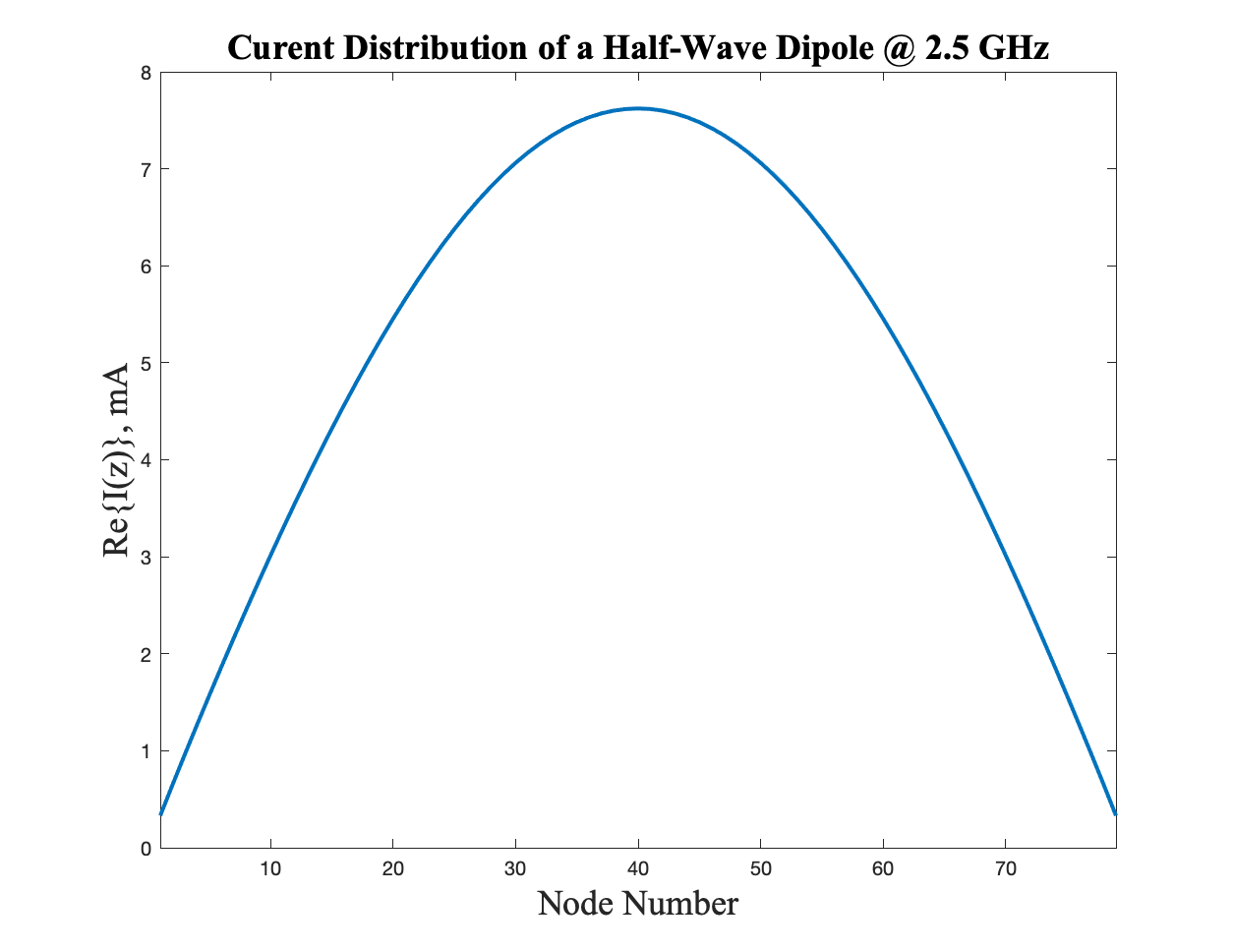
The following was generated by my code for an 81 node (79 basis function) \(\lambda/2\) dipole operated at a resonance of 2.5 GHz:

MATLAB generated current distribution.

This result is exactly what we expect for the wire that was designed. As we see, the current takes the form of a standing wave with nodes at the endpoints, and an anti-node (maximum) right at the feed-point of the antenna.

Input Impedance

The graph of the input impedance over a range of frequencies is shown as follows:

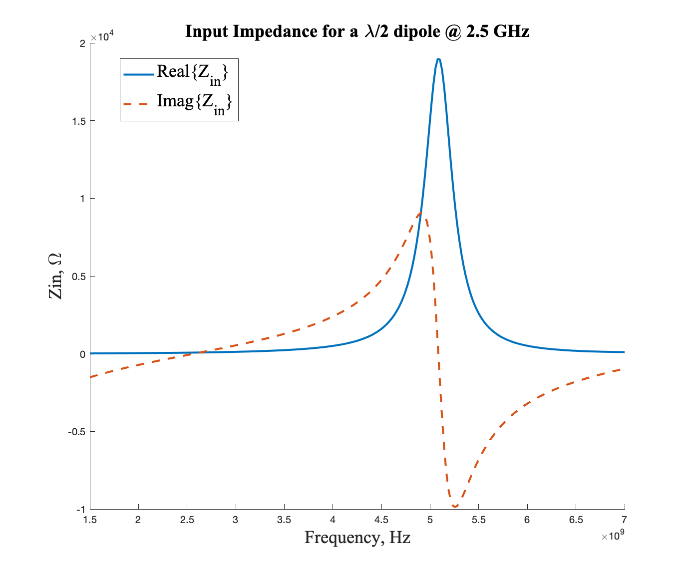Input impedance of the antenna vs. frequency.

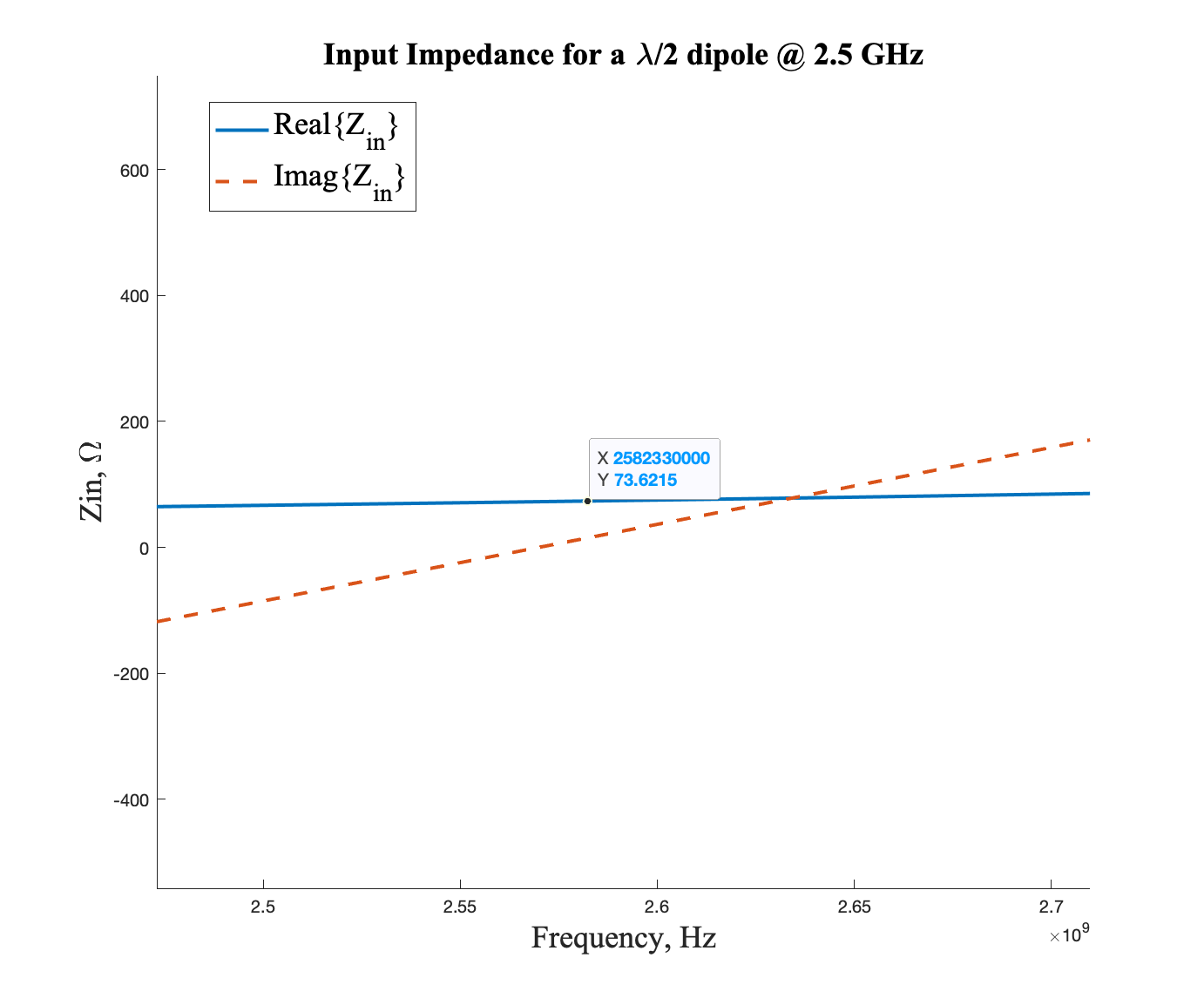Enlarged ~ input impedance of the antenna vs. frequency

We can see that for this half-wave dipole with 81 nodes, resonance occurs around \(2.56\) GHz, with a radiation resistance of \(Z_{in} = 73.6215 \Omega\), which is what we expect. Since the radius of the wire is not infinitesimally thin, the resonance value does not occur at the exact design frequency. Additionally, the number of basis functions affects convergence, which will be studied next.

Convergence to Analytic Radiation Resistance and Dependence on Meshing Parameters

The number of nodes affects how many intervals Maxwell’s equations will be solved over. Theoretically speaking, the smaller the interval the more accurate we expect the results to be. This section explores the convergence to the true $R_r$ value of $73 \Omega$ vs. the number of basis functions employed on the mesh. The following graph depicts this process

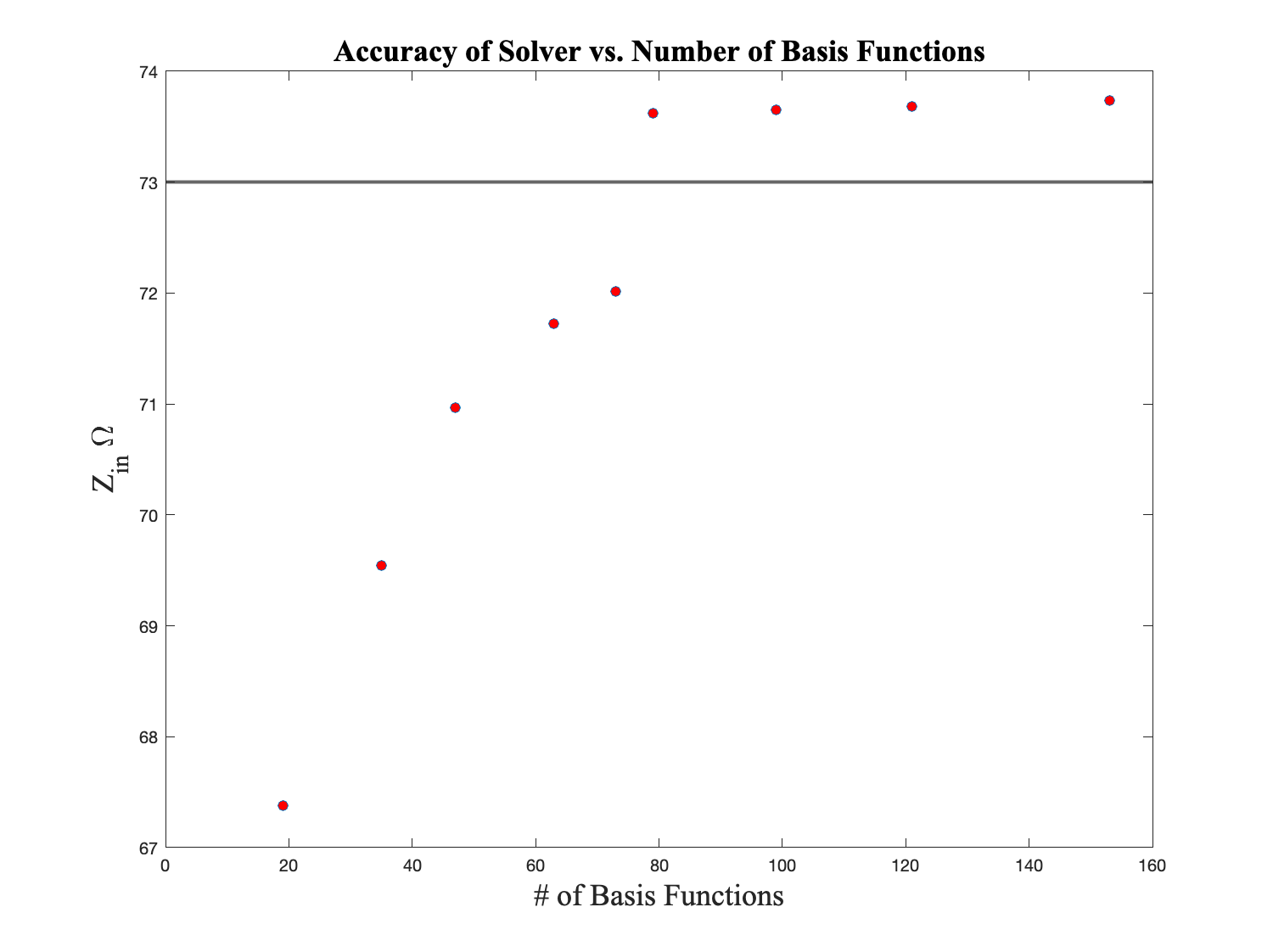Radiation resistance convergence vs. frequency.

We can see that at the number of nodes increases, there is slight fluctuation around 73.5, which tells us that the value is pretty much converged to where it will stay.

Characteristic Mode Tracking

Characteristic mode theory is a frequency based modal analysis for radiating systems. The modes of a radiating system can be deduced via the impedance matrix derived from the Method of Moments. The CMs arise from the generalized eigenvalue problem given in ³ as

\[\mathcal{X}(\mathbf{I_n}) = \lambda_n\mathcal{R}(\mathbf{I_n}) \tag{25}\]

where \(\mathcal{X}\) and \(\mathcal{R}\) are the imaginary and real part of the impedance matrix \(\mathcal{Z}\), while \(\mathbf{I_n}\) is the modal expansion coefficient for the given basis function. Characteristic modes are of interest because they, “minimize the ratio of the net reactive power \(\omega(W_m − W_e)\) to radiated power \(P_r\).

Numerically, this can be a complex problem as the impedance matrix is generally very large and dense. For small wire antennas with a discretization of \(<100\) segments, it is reasonable and easy to compute. In general CM tracking using the \(eigs()\) function in MATLAB will run at \(\mathcal{O}(n^3)\) since matrix inversion is required. The following depicts the first 6 modes for an 81 basis function representation for a \(\lambda/2\) dipole with a resonance frequency of \(2.5\) GHz.

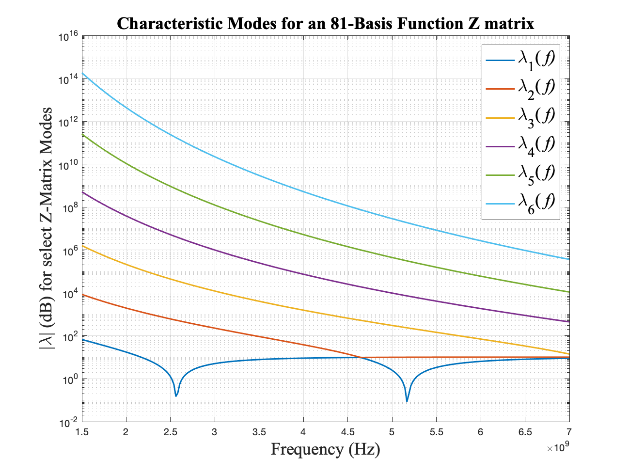Characteristic Modes vs. Frequency.

It is seen from Figure 8 that the smallest magnitude eigenvalue has a dual-band modal resonance at $2.56$ GHz and $5.16$ GHz. Each mode converges to a magnitude of $10$ dB. At these modal resonance frequencies, power is mostly radiating from the structure as opposed to being stored in the reactive near field. Many other insights can be derived from careful analysis of characteristic modes, and it is a rapidly re-emerging topic in the field of electromagnetics and antenna design.

Biblography

1. M. Gustafsson, K. Schab, L. Jelinek, and M. Capek. Upper bounds on absorption and scattering. 2019. ↩

2. Gary A. Thiele, Walter L. Stutzman. Antenna Theory and Design, Third Edition. Wiley, 2012. ↩ ↩²

3. Miloslav Capek, Paul Hazdra, Michael Masek, and Vit Losenicky. Analytical representation of characteristic mode decomposition. IEEE Transactions on Antennas and Propagation, vol. 65, no. 2, 2017, pp. 713–720, 2017. ↩