
Antenna Array Background
Overview
Antenna arrays, also known as phased arrays or simply arrays, are configurations of multiple antennas that work together as a single system to transmit or receive electromagnetic signals. These arrays are designed to enhance the performance of radio communication systems by manipulating the direction, shape, and strength of the electromagnetic waves they emit or receive.
As noted in 1 , there are at least five knobs that can be tuned to determine and control an antenna array’s characteristics:
- the geometrical configuration of the overall array (linear, circular, rectangular, spherical, etc.)
- the relative displacement between the elements
- the excitation amplitude of the individual elements
- the excitation phase of the individual elements
- the relative pattern of the individual elements
Antenna arrays now find use in a wide variety of wireless fields, but like many pioneering electromagnetic/communication system technologies its origin can be traced back to military applications 2. The concept of antenna arrays dates back to the early 20th century. One of the earliest notable applications was in World War II, where radar systems used simple forms of antenna arrays to detect and locate enemy aircraft. Engineers and scientists quickly realized the potential of arrays for various applications beyond military use and are now a salient feature of modern communication systems.
Some examples of of the key ways antenna arrays are useful today:
Beamforming: Antenna arrays can electronically steer their radiation pattern, allowing them to focus their signal energy in specific directions. This beamforming capability is crucial in wireless communication systems (e.g., 5G & WiFi) to establish reliable connections and increase network capacity.
Spatial Diversity: Arrays can improve signal reception in challenging environments by exploiting spatial diversity. When signals are received via multiple antennas, the system can select the best-quality signal or combine them to mitigate fading and interference.
MIMO Technology: Multiple Input Multiple Output (MIMO) technology, which uses antenna arrays at both the transmitter and receiver, significantly improves the capacity and reliability of wireless communication systems, such as Wi-Fi and LTE.
Radar Systems: Modern radar systems, including weather radar and automotive radar (for autonomous vehicles), use phased arrays to scan and track objects with high precision and speed.
Satellite Communication: Phased array antennas are employed in satellite communication systems to track and communicate with satellites in geostationary or low Earth orbit, ensuring continuous coverage and reducing the need for mechanical dish repositioning
Additionally, antenna arrays will play an integral role in next generation cellular technologies (6G, reconfigurable intelligent surfaces), radio astronomogy, wireless power transfer, and many more exciting developments. These notes will provide a brief technical background with some examples to demonstrate the theory in practice.
Array Fundamentals
Two-Element Array
The simplest way to understand the antenna array principle is to consider the case of two identical antennas placed at some sepatation $d$ from each other positioned along the $z$-axis. Eventually we’d like to consider more complex patterns with $N$-elements, and this simple 2-element case can eventually be extrapolated to that scenario.
Consider the antenna under investigation to be an array of two infinitesimal horizontal dipoles as shown in the Fig. 1 below:
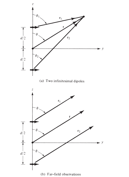 Figure 1 - A 2-element dipole antenna array 1.
Assuming no coupling between the two antenna elements, the total fied is given by:
\[\mathbf{E}_t=\mathbf{E}_1+\mathbf{E}_2=\hat{\mathbf{a}}_\theta j \eta \frac{k I_0 l}{4 \pi}\left\{\frac{e^{-j\left[k r_1-(\beta / 2)\right]}}{r_1} \cos \theta_1+\frac{e^{-j\left[k r_2+(\beta / 2)\right]}}{r_2} \cos\theta_2\right\} \tag{1}\]In this case, $\beta$ is the phase difference between the antennas, and the magnitude of each excitation source is the same. Making the far-field approximation (bottom of Fig. 1) we have that
\[\left.\begin{array}{l} \theta_1 \simeq \theta_2 \simeq \theta \\ r_1 \simeq r-\frac{d}{2} \cos \theta \\ r_2 \simeq r+\frac{d}{2} \cos \theta \\ r_1 \simeq r_2 \simeq r \end{array}\right\} \text { far-field approximation } \tag{2}\]Applying the FF approximation, Eq. (1) reduces to
\[\begin{array}{l} \mathbf{E}_t=\hat{\mathbf{a}}_\theta j \eta \frac{k I_0 l e^{-j k r}}{4 \pi r} \cos \theta\left[e^{+j(k d \cos \theta+\beta) / 2}+e^{-j(k d \cos \theta+\beta) / 2}\right] \\ \mathbf{E}_t=\hat{\mathbf{a}}_{\theta j} j \eta \frac{k I_0 l e^{-j k r}}{4 \pi r} \cos \theta\left\{2 \cos \left[\frac{1}{2}(k d \cos \theta+\beta)\right]\right\} \tag{3} \end{array}\]By looking at Eq. (3), it can be observed that the total field due to the array is equal to the pattern of a single element positioned at the origin times some scaling factor. This is known as the array factor.
The array factor of any two-element array is written as:
\[AF = 2\cos[\frac{1}{2}(kd\cos\theta+\beta)] \tag{4}\]\((\mathrm{AF}) e^{j \psi}=e^{j \psi}+e^{j 2 \psi}+e^{j 3 \psi}+\cdots+e^{j(N-1) \psi}+e^{j N \psi} \tag{5}\) We see that the AF is a function of antenna geometry and phase difference between the elements. In general, each array will have its own array factor that is a function of the number of elements, relative magitude/phases, topology, and relative spacings.
N-Element Arrays
The analysis of N-element arrays is similar to that of the simple 2-element case.
Consider Fig. 2 below where all antenna elements have te same amplitude and each successive element has a $\beta$ degree current phase lead relative to the other elements in the array.
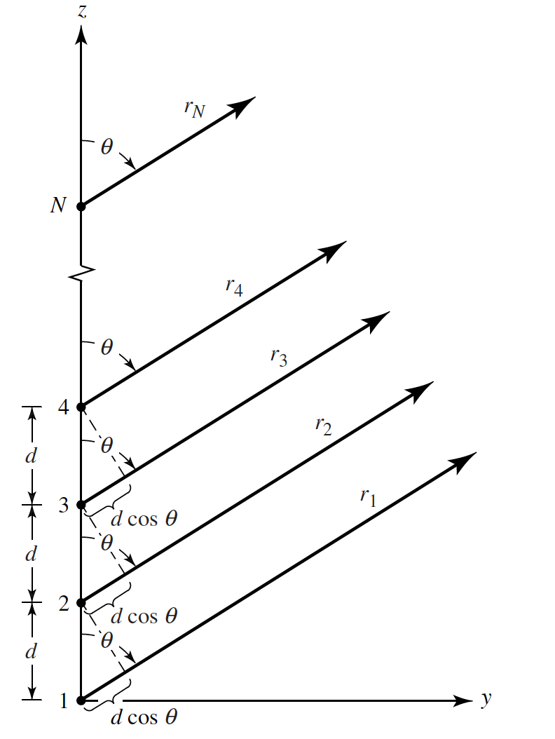 Figure 2 - An N-element uniform antenna array 1.
This is known as a uniform array. The array factor is obtained by analyzing the structure as a collection of point sources. Note that even if the actual elements are not isotropic sources, the total field can be resolved by multiplying the AF of the isotropic sources by the field of a single elements of the array. This is the pattern multiplication principle for uniform arrays, and the AF is given by:
\[\begin{array}{l} \mathrm{AF}=1+e^{+j(k d \cos \theta+\beta)}+e^{+j 2(k d \cos \theta+\beta)}+\cdots+e^{j(N-1)(k d \cos \theta+\beta)} \\ \mathrm{AF}=\sum_{n=1}^N e^{j(n-1)(k d \cos \theta+\beta)} \end{array} \tag{6}\]We can write this in a simpler form as:
\[\mathrm{AF}=\sum_{n=1}^N e^{j(n-1) \psi} \tag{7}\]where $\psi=k d \cos \theta+\beta$
In a uniform array, the AF is controlled by selecting the appropriate phase $\psi$ between the different elements. Note that in a non-uniform array, the amplitude is another knob that can be varied amongst elements to control the AF.
Another nice way to write the AF with the reference point as the center of the array is as follows (using properties of complex exponentials to rewrite the form into a form with only the sine term):
\[\mathrm{AF}=\left[\frac{\sin \left(\frac{N}{2} \psi\right)}{\sin \left(\frac{1}{2} \psi\right)}\right] \tag{8}\]To find the nulls of the array, one needs to simply find the arguments which cause the AF to equal $0$. For example, to find the nulls of Eq. 9, we have that
\[\begin{aligned} \sin \left(\frac{N}{2} \psi\right)=\left.0 \Rightarrow \frac{N}{2} \psi\right|_{\theta=\theta_n}= \pm n \pi \Rightarrow \theta_n & =\cos ^{-1}\left[\frac{\lambda}{2 \pi d}\left(-\beta \pm \frac{2 n}{N} \pi\right)\right] \\ n & =1,2,3, \ldots \\ n & \neq N, 2 N, 3 N, \ldots \end{aligned} \tag{9}\]and the maximum value is given as
\[\begin{aligned} \frac{\psi}{2}=\left.\frac{1}{2}(k d \cos \theta+\beta)\right|_{\theta=\theta_m}= \pm m \pi \Rightarrow \theta_m & =\cos ^{-1}\left[\frac{\lambda}{2 \pi d}(-\beta \pm 2 m \pi)\right] \\ m & =0,1,2, \ldots \end{aligned}\]Broadside Arrays
Broadside arrays are defined as those with a maximum radiation directed normal to the axis of the array. For a broadside array, it is desired to have the direction of maximum radiation directed towards $\theta_0 = 90^{\circ}$. This means that th maximum of the array factor occurs when
\[\psi = kdcos\theta + \beta|_{\theta=90^{\circ}} = \beta = 0 \tag{7}\]From Eq. 7 it is observed that to have the maximum of the AF for a uniform linear array with radiation maximized towards broadside that all elements in the ULA should have the same phase and amplitude excitation. The spacing between the elements can take on any value, however, to ensure that there are no grating lobes (undesired maxima in the radiation pattern) the separaton should not equal multiples of a wavelengths ($d \neq n\lambda$, $n = 1, 2, 3,… $). It can be seen that for a broadside ULA when $\beta=0$, if $d = n\lambda$ then $\psi=kdcos\theta+\beta=2\pi n cos\theta = \pm 2n\pi$. This causes the radiation pattern to have a maximum in the end-fire direction in addition to broadside. Thus, to avoid this condition the maximum spacing of the antenna elements should always be $d_{\text{max}} < \lambda $.
An example of a standard broadside pattern and a broadside pattern with additional grating lobes is shown in Fig. 3 below:
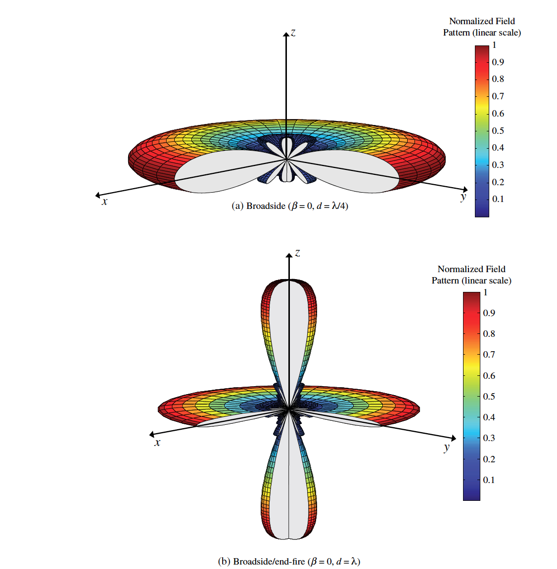 Figure 3 - 3D radiation pattern plot for a broadside and broadside with endfire grating lobes 1.
Endfire Arrays
Endfire arrays are similar to broadside arrays, however the desired direction of maximum radiation in the endfire case is along the direction of the array itself $\theta_0 = 0^{\circ}$ or $\theta_0 = 180^{\circ}$.
For maximum radiation occuring along $\theta_0 = 0^{\circ}$,
\[\psi = kdcos\theta + \beta|_{\theta=0^{\circ}} = kd+ \beta = 0 \rightarrow \beta = -kd \tag{8}\]For maximum radiation occuring along $\theta_0 = 180^{\circ}$,
\[\psi = kdcos\theta + \beta|_{\theta=180^{\circ}} = -kd+ \beta = 0 \rightarrow \beta = kd \tag{9}\]Note that for end-fire arrays, in order to avoid grating lobes the condition for maximum element spacing should be such that $d_{\text{max}}< \lambda /2$.
An example amplitude radiation pattern for both $0^{\circ}$ and $180^{\circ}$ is shown below.
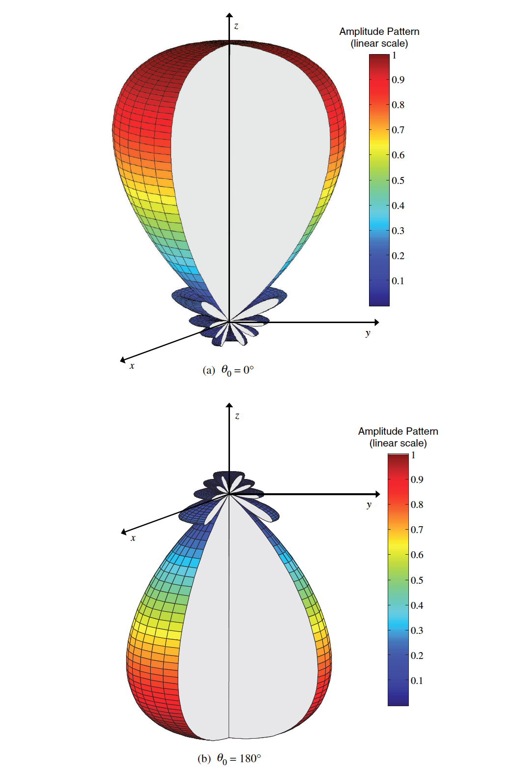 Figure 4 - 3D radiation pattern plot for endfire arrays directed towards $0^{\circ}$ and $180^{\circ}$. ($N=10$, $d=\lambda/4$) 1.
Scanning & Pattern Control Principles
In antenna array systems, the method for controlling the beam direction is based upon manipulation of the phase excitation delta between the elements of the antenna array. Additionally, the sidelobe level and beam shape can be controlled by manipulation of the amplitude distribution. This is done by weighting the signals impigning on each antenna element. There are many weighting schemes that can be used depending on the design objectives. A weight is simply a multiplication factor applied to the signals on each antenna element.
The phased array (discussed in the next section) is the simplest and most widely employed type of array system. In practice, the phased array can be combined with amplitude weighted systems to produce an array with precise direction, beam shape, and side lobes.
One of the modern approaches to weighting is the so-called adaptive weighting based on least mean-square error (LMS) which dynamically adapts the weights based on received signal characteristics in order to improve the performance of the antenna array system. This is highlighted in another post on smart antenna systems.
Phased Arrays
Given that the radiation pattern can be designed to orient broadside and endfire to the antenna array, it’s plausible to assume that the radiation pattern can be orinted in any direction to form a scanning (phased) array. To control the maximum radiation of the array between $\theta_0 (0^{\circ} \leq $ $\theta_0 \leq 180^{\circ})$, the phase excitation delta between the antenna elements must be adjusted such that
\[\psi = kdcos\theta + \beta|_{\theta=theta_0^{\circ}} = kdcos\theta_0 + \beta = 0 \rightarrow \beta = -kdcos\theta_0 \tag{8}\]From Eq. 8, it is observed that by changing the phase difference between the elements, the maximum radiation can be set in any desired direction. In practice, this continuous phase shifting can be carried out by a dedicated phase shifter IC or by the use of ferrite or diode phase shift circuits.
Planar Arrays
The planar array involves the placement of indiviual array elements along a grid to form a planr array - this provides additional conrol parameters to shape the behavior of the array and offers additional radiation benefits such as more symmetrical patterns with lower side lobe levels. Additionally, planar arrays allow the main beam to be scanned towards any point in space and allow for applications such as point tracking radar, electronic search systems, remote sensing, and high frequency communication systems with extended range.
Array Factor
For a planar array with M elements placed along the x-axis (see Fig. 5), the array factory can be written as
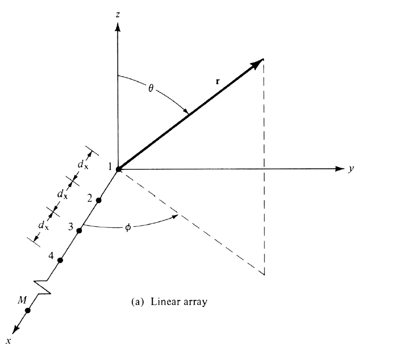 Figure 5 - Linear array geometry with elements oriented along the $x$-axis 1.
with $I_{m1}$ the excitation coefficient for each element in the array, $d_x$ is the element spacing, and $\beta_x$ the phase shift between the elements. Placing $N$ of these arrays next to each other in the $y$-direction a distance $d_y$ apart with phase shift $\beta_y$ forms a rectaungluar array as shown below in Fig. 6.
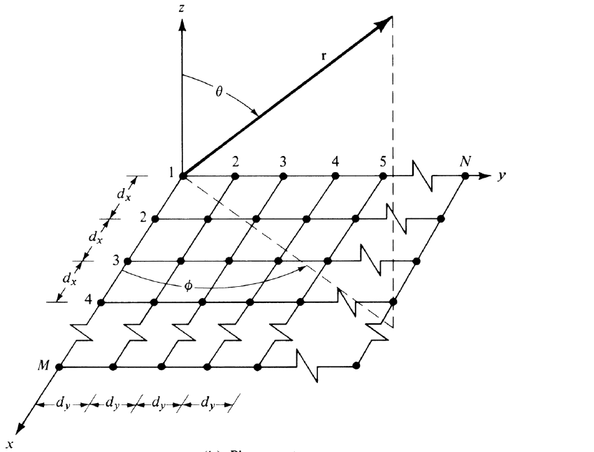 Figure 6 - Planar array geometry 1.
The array factor of the entire planar array is written as:
\[\mathrm{AF}=S_{xm}S_{yn}=\sum_{n=1}^N I_{1 n}\left[\sum_{m=1}^M I_{m 1} e^{j(m-1)\left(k d_x \sin \theta \cos \phi+\beta_x\right)}\right] e^{j(n-1)\left(k d_y \sin \theta \sin \phi+\beta_y\right)} \tag{10}\]which indicates that the rectangular array pattern is the product of the $x$ and $y$ directed array factors. Similar conditions exist to the 1D linear arrays to avoid the formation of grating lobes, namely the element spacing for the $x$ and $y$ directions must be less than $\lambda/2$.
For rectangular arrays, the major and grating lobes of $S_{xm}$ and $S_{ym}$ are located at the following points in the phase excitation delta argument:
\[\begin{array}{l} k d_x \sin \theta \cos \phi+\beta_x= \pm 2 m \pi \quad m=0,1,2, \ldots \\ k d_y \sin \theta \sin \phi+\beta_y= \pm 2 n \pi \quad n=0,1,2, \ldots \end{array} \tag{11}\]Note that the phases for the $x$ and $y$ directions are independent of each other and can be tuned such that they have different maxima directions. That being said, most applications desire to have the main beams for $S_{xm}$ and $S_{yn}$ intersect with each other and point in the same direction. In other words, it is desire to have one beam pointed in the $\theta = \theta_0$ and $\phi = \phi_0$ direction. For this to occur, it is required that the excitation phase delta between the array elements in the $x$ and $y$ directions meet the following conditions:
\[\begin{array}{l} \beta_x=-k d_x \sin \theta_0 \cos \phi_0 \\ \beta_y=-k d_y \sin \theta_0 \sin \phi_0 \end{array} \tag{12}\]Nonuniform Amplitude Arrays
Thus far, only linear arrays with uniform spacing, amplitude, and progressive phase shift have been considered. In practice, the desried characteristics of an antenna array may often necessitate nonuniform design parameters in order to achieve desired array characteristics such as directivity, beamwidth, side-lobe level, and efficiency. This section will highlight broadside arrays with nonuniform amplitude distributions.
There are three primary amplitude distributions in antenna array theory:
- uniform
- binomial
- Dolph-Tschebyscheff
Of the three typs, unform distributions offer the smallest half-power beamwidth potential which is followed by the Dolph-Tschebyscheff and binomial arrays. On the flip side, binomial distribution offers the smallest SLL which is followed by Dolph-Tschebyscheff and uniform arrays. One of the key tradeoffs of antenna array design is the compromise between beamdwidth and SLL. Of the three distributions, the tapered Dolph-Tschebyscheff distribution producs the best tradeoff between beamwidth and SLL.
Nonuniform Array Factor
For analysis purposes, only a linear 1D array with an even $2M$ elements will be considered (see Fig. 7).
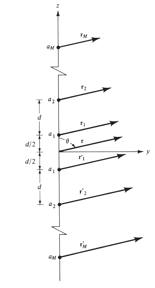 Figure 7 - Nonuniform linear array with an even amount of elements 1.
The AF can be written as
\[\begin{aligned} (\mathrm{AF})_{2 M}=a_1 e^{+j(1 / 2) k d \cos \theta} & +a_2 e^{+j(3 / 2) k d \cos \theta}+\cdots \\ & +a_M e^{+j[(2 M-1) / 2] k d \cos \theta} \\ & +a_1 e^{-j(1 / 2) k d \cos \theta}+a_2 e^{-j(3 / 2) k d \cos \theta}+\cdots \\ & +a_M e^{-j[(2 M-1) / 2] k d \cos \theta} \\ (\mathrm{AF})_{2 M} & =2 \sum_{n=1}^M a_n \cos \left[\frac{(2 n-1)}{2} k d \cos \theta\right] \end{aligned} \tag{13}\]which can be expressed in normalized form as
\[(\mathrm{AF})_{2 M}(\text { even })=\sum_{n=1}^M a_n \cos [(2 n-1) u] \tag{14}\]The amplitude excitation of the array’s center element is represented by the coefficient $2a_{1}$.
Dolph-Tschebyscheff Broadside Arrays
This section will highliught the parameters and design procedure of the Dolph-Tschebyscheff array. The Dolph-Tschebyscheff is a hybrid of the uniform and binomial distributed arrays, and therefore offers a middleground to the SLL and beamwidth. Often there is a desire to lower the highest sidelobes in the pattrn at the expense of raising the lower sidelobs. This optimal SLL occurs when all sidelobes are equal in magnitude. The Dolph-Tschebyscheff accomplishes this and allows for the minimum possible null-null beamwidth.
As indicated by the name, the Dolph-Tschebyscheff array has excitation coefficients that are derived from the Tschebyscheff polynomials. In the extreme case, the Dolph-Tschebyscheff distributed array reduces to the binomial distributed array. Referring to Eq. 14, the array factor consists of a linear combination of complex exponentials with the largest harmonic being one less than the total number of elements in the array. Each term consists of an interger tines some fundamental frequency, and can be decomposed and rewritten as a series of cosine functions with the fundamental frequency as an argument. This is shown below in Eq. 15:
\(\begin{array}{ll} m=0 & \cos (m u)=1 \\ m=1 & \cos (m u)=\cos u \\ m=2 & \cos (m u)=\cos (2 u)=2 \cos ^2 u-1 \\ m=3 & \cos (m u)=\cos (3 u)=4 \cos ^3 u-3 \cos u \\ m=4 & \cos (m u)=\cos (4 u)=8 \cos ^4 u-8 \cos ^2 u+1 \\ m=5 & \cos (m u)=\cos (5 u)=16 \cos ^5 u-20 \cos ^3 u+5 \cos u \\ m=6 & \cos (m u)=\cos (6 u)=32 \cos ^6 u-48 \cos ^4 u+18 \cos ^2 u-1 \\ m=7 & \cos (m u)=\cos (7 u)=64 \cos ^7 u-112 \cos ^5 u+56 \cos ^3 u-7 \cos u \\ m=8 & \cos (m u)=\cos (8 u)=128 \cos ^8 u-256 \cos ^6 u+160 \cos ^4 u-32 \cos ^2 u+1 \\ m=9 & \cos (m u)=\cos (9 u)=256 \cos ^9 u-576 \cos ^7 u+432 \cos ^5 u-120 \cos ^3 u+9 \cos u \end{array} \tag{15}\) Note that the above form is found applying Euler’s identity to Eq. 14. The full form of the Dolph-Tschebyscheff polynomial representation including the generating polynomial forms can be found in 1.
When designing Dolph-Tschebyscheff arrays, often it is assumed that the number of elements, spacing, major-to-minor lobe intensity ratio $R_0$ are known and thus the tasks breaks down into determining the excitation coefficients and the array factor. The full design procedure is highlighted in Section 6.8.3 of 1.
Design Considerations
Designing phased array antenna systems requires careful consideration of the number of elements, element spacing, excitation amplitude/phase, half-power beamwidth (hpbw), directivity, and side lobe level (SLL). For phased (scanning) array systems, the principle of beam control is the manipulation of progressive phase excitation deltas between the elements of the array. Additionally, control of the amplitude excitation can be used for adjustment of the pattern beamwidth and SLL (note that SLL is a tradeoff from beamwidth, where designing for a low SLL correspondingly decreases the the HPBW and increases the directivity of the array.) It’s important to have a low SLL is most systems. Two practical problems from high sidelobes could be increases interference from base station transmit antennas onto other devices, as well as false object detection in radar systems due to ranging signals being picked up by sidelobes at a level at a level above the detection threshold.